Longitudinal Traffic model: The IDM |
 |
In this simulation, we have used the
Intelligent-Driver Model (IDM) to simulate the longitudinal
dynamics,
i.e., accelerations and braking
decelerations of the drivers.
Model Structure
The IDM is an microscopic traffic flow model, i.e.,
each vehicle-driver combination constitutes an active "particle" in
the simulation. Such model characterize the traffic state at any
given time by the positions and speeds of all simulated vehicles. In
case of multi-lane traffic, the lane index complements the state
description.
More specifically, the IDM is a car-following model. In
such models, the decision of any driver to accelerate or to
brake depends only on his or her own speed, and
on the position and speed of the "leading vehicle" immediately ahead.
Lane-changing decisions, however, depend on all neighboring
vehicles (see the lane-changing model MOBIL).
The model structure of the IDM can be described as follows:
- The influencing factors (model input) are the own speed v, the
bumper-to-bumper gap s to the leading vehicle, and the relative
speed (speed difference) Delta v of the two vehicles (positive when approaching).
- The model output is the acceleration dv/dt chosen by the driver
for this situation.
- The model parameters describe the driving style, i.e.,
whether the simulated driver drives slow or fast, careful or
reckless, and so on: They will be described in
detail below.
Model Equations
The IDM model equations read as follows:
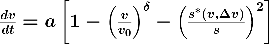
where

The acceleration is divided into a "desired" acceleration
a [1− (v/v0)delta] on a free
road, and braking decelerations induced by the front vehicle.
The acceleration on a free road decreases from the initial
acceleration a to zero when approaching the "desired speed"
v0.
The braking term is based on a comparison between the "desired
dynamical distance" s*, and the actual gap s to the
preceding vehicle. If the actual gap is approximatively equal to
s*, then the breaking deceleration essentially
compensates the free acceleration part, so the resulting
acceleration is nearly zero. This means, s*
corresponds to the gap when following other vehicles in steadily
flowing traffic.
In addition, s* increases dynamically when
approaching slower vehicles and decreases when the front vehicle
is faster. As a consequence,
the imposed deceleration increases with
- decreasing distance to the front vehicle (one wants to maintain a
certain "safety distance")
- increasing own speed (the safety distance increases)
- increasing speed difference to the front vehicle (when approaching
the front vehicle at a too high rate, a dangerous situation
may occur).
The mathematical form of the IDM model equations is that of
coupled ordinary differential equations:
- They are differential equations since, in one equation, the dynamic
quantities v (speed) and its derivative dv/dt (acceleration) appear
simultaneously.
- They are coupled since, besides the speed v, the equations also
contain the speed vl=v− Delta v of the leading
vehicle. Furthermore, the gap s obeys its own kinematic equation,
ds/dt=− Delta v
coupling the gap s to the speeds of the two vehicles.
Model Parameters
The IDM has intuitive parameters:
- desired speed when driving on a free road, v0
- desired safety time headway when following other vehicles, T
- acceleration in everyday traffic, a
- "comfortable" braking deceleration in everyday traffic, b
- minimum bumper-to-bumper distance to the front vehicle, s0
- acceleration exponent, delta.
In general, every "driver-vehicle unit" can have its individual parameter
apply set, e.g.,
- trucks are characterized by low values of v0, a, and b,
- careful drivers drive at a high safety time headway T,
- aggressive ("pushy") drivers
are characterized by a low T in connection
with high values
of v0, a, and b.
Often two different types are sufficient to show the main phenomena.
The standard parameters used in the simulations are the following:
| Parameter |
Value Car |
Value Truck |
Remarks |
| Desired speed v0 |
120 km/h |
80 km/h |
For city traffic, one would adapt the desired
speed while the other parameters essentially can be left
unchanged.
|
| Time headway T |
1.5 s |
1.7 s |
Recommendation in German driving schools: 1.8 s; realistic values
vary between 2 s and 0.8 s and even below. |
| Minimum gap s0 |
2.0 m |
2.0 m |
Kept at complete standstill, also in queues that are caused by red
traffic lights. |
| Acceleration a |
0.3 m/s2 |
0.3 m/s2 |
Very low values to enhance the formation of stop-and go
traffic. Realistic values are 1-2 m/s2 |
| Deceleration b |
3.0 m/s2 |
2.0 m/s2 |
Very high values to enhance the formation of stop-and go
traffic. Realistic values are 1-2 m/s2 |
Simulation of the Model
Simulation means to numerically "integrate", i.e., approximatively
solve the coupled differential
equations of the model. For this, one defines a finite numerical
update time interval Δt, and integrates over this time
step assuming constant accelerations. This so-called ballistic
method reads
| new speed: | v(t+Δt)=v(t) + (dv/dt) Δt, |
| new position: |
x(t+Δt)=x(t)+v(t)Δt+1/2 (dv/dt) (Δt)2, |
| new gap: |
s(t+Δt)
=xl(t+Δt)− x(t+Δt)− Ll. |
where dv/dt is the IDM acceleration calculated at time t,
x is the position of the front bumper, and Ll the
length of the leading vehicle.
For the Intelligent-Driver Model, any update time steps below 0.5
seconds will essentially lead to the same result, i.e., sufficiently approximate
the true solution.
Strictly speaking, the model is only well defined if there is a
leading vehicle and no other object impeding the driving. However,
generalizations are straightforward:
- If there is no leading vehicle and no other obstructing object ("free
road"), just set the gap to a very large value such as
1000 m (The limes gap to infinity is well-defined for any meaningful
car-following model such as the IDM).
- If the next obstructing object is not a leading vehicle but a red
traffic light or a stop-signalized intersection, just model the
red light or the stop sign by a standing virtual
vehicle of length zero positioned at the stopping line. When
simulating a transition to a green light, just eliminate the virtual
vehicle. (See the szenario "traffic Lights")
- If a speed limit (either directly by a sign or indirectly, e.g.,
when crossing the city limits) becomes effective, reduce the desired
speed, if the present value is above this limit (scenario
"Laneclosing"). Likewise, reduce
the desired speed of trucks in the presence of gradients (scenario
"Uphill Grade")
Special Case of Stopped Vehicles
For vehicles approaching
an already stopped vehicle or a red traffic light, the ballistic
update method as described above will lead to negative
speeds whenever the end of a time integration interval is not exactly
equal to the true stopping time (of course, there is always a mismatch).
Then, the ballistic method has to be generalized to
simulate following approximate dynamics:
If the true stopping
time is within an update time interval, decelerate at constant
deceleration (dv/dt) to a complete stop and remain at standstill
until this interval has ended.
Furthermore, it may happen that the actual gap of a stopped vehicle s is slightly
below the minimum gap s0, in which case the
unchanged IDM would give a negative acceleration, hence a negative
velocity in the next time step. In most cases, however, real drivers
will just keep that somewhat too low gap until the leader drives
again rather than driving backwards.
Both special cases can be implemented by following rules
which are generally applicable to integrating any time-continuous
car-following model, not just the IDM:
| At least one of the above situations applies if: |
v(t) + (dv/dt) Δt < 0, |
| new speed in this case: |
v(t+Δt)=0, |
| new position in this case: |
x(t+Δt)=x(t) − 1/2 v2(t) / (dv/dt), |
| new gap: |
s(t+Δt)
=xl(t+Δt)− x(t+Δt)− Ll. |
Notice that − 1/2 v2(t) / (dv/dt) is greater than
zero if the special cases apply.
Further information:
Martin Treiber